3.8. Dynamic stochastic modelling: infiltration model¶

3.8.1. Introduction¶

Important note: questions in this section are NOT available in Blackboard so please answer in a text document that you hand in afterwards. This section is also not part of the Land Surface Process Modelling course.

3.8.2. Model structure and field data¶

In the exercises, you will use a rainfall-runoff model simulating the Hortonian overland flow during a single rainstorm event. This section provides a short introduction to the model. Note that you need at least 2 GB diskspace for the exercises.

You will use data from an approximately rectangular 7500 m2 sandy loam hillslope with a vineyard, located in the Ouveze river basin, S. France. The model simulates rainfall, infiltration and overland flow. Interception is ignored here for reasons of simplicity (note that it is rather small anyway on a vineyard), as is surface storage.

Open the model runoff.py and have a look at the code. Run the model.

Display the input maps

aguila dem.map + ldd.map out.map + ldd.map &

The map dem.map is the digital elevation model of the modelling area, ldd.map is the local drain direction map with the drainage directions. out.map gives the ouflow location of the catchment.

Rainfall is modelled as a block rainstorm (constant rainfall at the start of the modelling period abruptly finishing half way):

aguila --timesteps=[1,360,1] --scenarios={1} p

Right-click on the legend for options and to open a timeseries (click on map to get the values for a location).

It is assumed that for each cell and each time step, infiltration capacity (m/h) equals the saturated conductivity ( $Z(\bf{s})$ , m/h). For each cell, the actual infiltration ( $I(\bf{s})$ , m/h) is the minimum value of the saturated conductivity and the water available for infiltration (m/h). The water available for infiltration is rainfall ( $P(\bf{s})$ , m/h) plus runon from upstream cells ( $R(\bf{s})$ , m/h). In an equation:

$I(\bf{s}) = min(K(\bf{s}),P(\bf{s}) + R(\bf{s}))$

where min(a,b) assigns the minimum value of a and b.

Runoff is routed using the Manning equation and the kinematic wave in downstream direction over the local drain direction map (ldd.map).

Saturated conductivity was measured at 10 locations on the hillslope using ring infiltrometer experiments. The average saturated conductivity was 0.05 m/h (n=10), which is quite normal for this type of soil. The standard deviation of the saturated conductivity data set was very high. In addition, discharge was measured at the outflow point of the catchment. With rainstorms having similar characteristics as the one used here, peak discharge was mostly about 0.02 m3/s. In the following exercises, you will try to simulate the discharge from the catchment, using an average K value of 0.02 m/h. The question is whether simulated discharge is in the same order of magnitude as measured discharge at the outflow point.

3.8.3. Deterministic modelling using mean K¶

The run with the model you did in the previous section was done using a saturated conductivity value of 0.05 m/h for all cells. This value is the same as the average value derived from the ring infiltrometre measurements. The question is how much runoff was generated by this run.

Let’s first have a look at the change through time of actual infiltration (m/h, the files i0000000.001, representing the first time step, up to i0000000.360, representing the last time step), runoff (m3/h, q0000000.001 up to q0000000.360), and actual infiltration as a percentage of the saturated conductivity (%, ip000000.001, ..). Note that these are written to the folder 1 but you do not need to care about this as it is indicated by scenarios in the aguila commane. Type from the folder where you were running the script:

aguila --timesteps=[1,360,1] --scenarios={1} i ip q + ldd.map &

and animate the maps. By right clicking on the legend you can open a time series view for a location on the map (just click on the map to change the location for which you want the time series). Note that the time step duration is 10 seconds. Click on the location of the outflow point to show the time series for that location.

Question

What is the peak discharge at the outflow point?

Correct answers: a.

Feedback:

0.000016 m3/h, which is a negligible amount

Question

Explain why such a small amount of discharge is generated (compared to the measured peak discharges for these kind of rainstorms).

Correct answers: Precipitation equals infiltration capacity and as a result everything infiltrates.

Feedback:

None

3.8.4. The stochastic model¶

The deterministic model used in the previous exercise does not generate runoff since it ignores spatial variation of saturated conductivity on the field. To give a more realistic representation of runoff, it is needed to include this spatial variation in our model. The problem is that there is insufficient data to represent this in a deterministic way, using a map with the actually occurring pattern of saturated conductivity on the field. The only way to solve the problem is to represent spatial variation of saturated conductivity as a stochastic variable, having a defined spatial probability distribution.

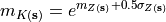
We assume a lognormal distribution of saturated conductivity by defining:

$K(\bf{s}) = e^{Z(\bf{s})}$

It is assumed that $Z(\bf{s})$ is a multivariable normal and stationary random spatial function. Thus, $Z(\bf{s})$ is defined by its expectation $m_{Z(\bf{s})}$ , its variance $\sigma_{Z(\bf{s})}$ and its spatial correlation structure. The spatial correlation structure could be defined by a variogram, but we will use a simplified approach here to create random fields very similar to thos created with a variogram.

The expectation (mean) of $K(\bf{s})$ is:

$m_{K(\bf{s})} = e^{m_{Z(\bf{s})} + 0.5 \sigma_{Z(\bf{s})}}$

Increasing $\sigma_{Z(\bf{s})}$ results in a probability distribution of $K(\bf{s})$ with both a higher variance and a higher skewness.

The model can be run in stochastic mode, using user defined spatial probability distributions of $K(\bf{s})$ . By modifying the following components of the script runoff.py, you can create scenario’s with different spatial probability distributions of $K(\bf{s})$ . In runoff.py you can define:

The number of Monte Carlo loops. The number of Monte Carlo loops is set in the following line at the upper part of the script:

nrSamples = 2

For instance, to run 50 loops, change the line to:

nrSamples = 50

Somewhat down, the value of $m_{K(\bf{s})}$ :

# mean of Z
mean = -2.9957

The value of $\sigma_{Z(\bf{s})}$ :

# variance of Z
var = 0.000001

The spatial correlation structure of $Z(\bf{s})$ . The random field is generated by drawing independent realizations for each pixel. This results in a random field corresponding to a variogram without range (only nugget). Spatially correlated versions are created by applying a smoothing window. This creates realizations with a spatial correlation structure. The larger the window, the larger the scale of variation (larger variogram range). This is set by the value of approximateRangeInPixels. A value of one corresponds to no spatial correlation (nugget only variogram), other possible values are 3, 5, 7, etc. It is now set to 1 (no spatial correlation):

# approximate range of random field (pixels), use 1, 3, 5, 7, ..
# note that 1 implies 'white noise', i.e. no spatial correlation
approximateRangeInPixels = 1

Using the information given above, make a copy of runoff.py and save it as runoff_stoch.py to run the model with:

50 Monte Carlo loops
white noise, no spatial correlation
a value of $\sigma_{Z(\bf{s})}$ of 1.0
an expectation (mean) of $K(\bf{s})$ of $m_{K(\bf{s})} = 0.05$ m/h

Question:

With the input values given above, what value needs to be used for $m_{Z(\bf{s})}$ ?

Correct answers: Use the equation in the course text to solve the equation. # mean of Z mean = -3.4957 # variance of Z var = 1.0

Feedback:

import shutil, sys
import pcraster.pcr as pcr
from pcraster import *
from pcraster.framework import *

# number of Monte Carlo samples
nrSamples = 50

# number of time steps
nrTimeSteps = 360

class Runoff(DynamicModel, MonteCarloModel):
  def __init__(self):
    DynamicModel.__init__(self)
    MonteCarloModel.__init__(self)
    setclone("clone.map")

  def initial(self):
    self.stepLength = 10               # Length of one timestep (s).

    dem = readmap("dem.map")
    self.landUnits = readmap("landunit.map")
    self.ldd = readmap("ldd.map")

    porosity = 0.4                     # Porosity (-).
    initMoistureContent = 0.05         # Initial moisture content.

    initInterceptStoreContent = 0      # (m, for area covered, 'Cov area').
    self.interceptCorrectionFactor = 1 # Correction factor canopy (0.046 * lai, is unit correct?).

    duration = 20                      # End of rainstorm (minutes).
    duration *= 60                     # End of rainstorm (s).

    self.precip = 0.017                # Precipitation (m).
    self.precip = (self.precip / duration) * self.stepLength # Per timestep (m).

    self.lastPrecipStep = duration / self.stepLength  # End of rainstorm (timesteps).

    self.cumPrecip = 0.0               # Cumulative rain (m).


    initStreamFlow = 0.000000000001    # Initial streamflow (m3/s).
    self.beta = 0.6                    # Beta.
    areaFraction = 1                   # Area fraction of all channels ???.
    self.nrChannelsPerCell = 1         # Nr of channels per cell ???.


    # random field generation
    # random field with expectation zero and standard deviation one
    whiteNoise = normal(1)
    # approximate range of random field (pixels), use 1, 3, 5, 7, ..
    # note that 1 implies 'white noise', i.e. no spatial correlation
    approximateRangeInPixels = 1 
    # number of pixels in window
    nrPixels = windowtotal(spatial(scalar(1)),approximateRangeInPixels*celllength())
    self.report(nrPixels,"np")
    # std corrector
    factor = sqrt(nrPixels)
    # random field with expectation zero, standard deviation one, and range
    # equal to approximateRange
    randomField = windowaverage(whiteNoise, approximateRangeInPixels*celllength()) * factor 
    self.report(randomField,"rf")

    # mean of Z
    mean = -3.4957
    # variance of Z
    var = 1.0

    # standard deviation of Z
    std = sqrt(var)
   
    # random field Z 
    Z = randomField * std + mean
    self.report(Z,"Z")
    
    ## INFILTRATION GREEN & AMPT 
    # Sat. inf. rate (m/h).
    ks = exp(Z)
    self.report(ks, "ks")
    #meanKs = areaaverage(ks, "clone.map")
    #self.report(meanKs, "meanKs")

    # initial surface water
    surfaceWater = 0.0                 # Total amount of water on surface (m).

    # Saturated conductivity (m/timestep).
    self.ksPerStep = (ks / 3600) * self.stepLength

    # Actual initial infiltration per timestep ('rate', m/timestep).
    self.initInfil = 0.00000001

    # Cumulative initial infiltration ('rate', m/timestep).
    self.cumInitInfil = 0.0000000001

    # Initial content of interception store (m, for area covered, 'Cov area').
    self.interceptStoreContent = initInterceptStoreContent

    lai = lookupscalar("lai.tbl", self.landUnits) # Leaf area index.

    # Maximum content of interception store (m, for area covered, 'Cov area'), m
    self.maxInterceptStoreContent = \
         max(0.935 + 0.498 * lai - 0.00575 * sqr(lai), 0.0000001) / 1000

    self.cumIntercept = 0.0       # Initial intercepted water, cumulative (m).

    # Area covered with vegetation.
    self.areaCovered = lookupscalar("cov.tbl", self.landUnits)

    # Amount of water in surface storage (m).
    self.surfaceWaterStorage = 0.0

    # Distance to downstream cell (m).
    self.distToDownstreamCell = max(downstreamdist(self.ldd), celllength())

    # Slope to downstream neighbour.
    slopeToDownStreamCell = \
         (dem - downstream(self.ldd, dem)) / downstreamdist(self.ldd)
    slope = cover(max(0.0001, slopeToDownStreamCell), 0.0001)

    self.discharge = initStreamFlow            # Initial streamflow (m3/s).
    self.cumQ = 0.0          # Cum amount of water added to streamflow (m).

    n = lookupscalar("n.tbl", self.landUnits)    # Manning's n.
    self.alphaTerm = (n / sqrt(slope)) ** self.beta        # Term for Alpha.
    self.alphaPower = (2.0 / 3) * self.beta      # Power for Alpha.

    waterDepth = 0.000000001                    # Initial water height (m).
    # Bottom width for routing (m).
    self.bottomWidth = areaFraction * celllength()

    # Initial approximation for Alpha.
    # Wetted perimeter (m) assume 8 channels per cell!
    wettedPerimeter = self.bottomWidth + 2 * self.nrChannelsPerCell * waterDepth
    self.alpha = self.alphaTerm * (wettedPerimeter ** self.alphaPower)

    # Conversion factor from m/step to m/h.
    self.stepToHour = 3600 / self.stepLength

  def dynamic(self):
    # Rain per timestep, constant rain (m/timestep).
    precipPerStep = ifthenelse(self.currentTimeStep() <= self.lastPrecipStep,
         scalar(self.precip), 0.0)

    # Rain (m/h).
    precipPerHour= precipPerStep * self.stepToHour * \
         scalar(defined(self.landUnits))
    self.report(precipPerHour, "p")

    self.cumPrecip = precipPerStep + self.cumPrecip   # Cumulative rain (m).

    # Intercepted water per timestep (m, spreaded over whole cell).
    intercept = precipPerStep * self.areaCovered

    # Intercepted water, cumulative (m, spreaded over whole cell).
    self.cumIntercept = self.cumIntercept + intercept

    # Amount in interception store (m, for area covered (for 'Cov area')).
    previousInterceptStoreContent = self.interceptStoreContent
    self.interceptStoreContent = self.maxInterceptStoreContent * (
         1 - exp((-self.interceptCorrectionFactor * self.cumPrecip) /
         self.maxInterceptStoreContent))

    # To interception store (m/timestep, for area covered (for 'Cov area')).
    toInterceptStore = self.interceptStoreContent - \
         previousInterceptStoreContent

    # To interception store (m/timestep, spreaded over whole cell).
    toInterceptStore = self.areaCovered * toInterceptStore

    # Throughfall (m, spreaded over whole cell).
    throughFall = intercept - toInterceptStore
    # self.report(throughFall, "TF")

    # Total net rain per timestep (m, spreaded over whole cell).
    netPrecip = throughFall + (precipPerStep - intercept)

    # Amount in interception store (m, spreaded over whole cell).
    interceptStoreContentCell = self.areaCovered * self.interceptStoreContent

    # Flow out off the cell (m/timestep).
    flowOutOfCell = (self.discharge * self.stepLength) / cellarea()
    # self.report(spatial(flowOutOfCell), "QR")

    # Total amount of water on surface, waterslice (m).
    surfaceWater = netPrecip + self.surfaceWaterStorage + flowOutOfCell
    # self.report(surfaceWater, "surfwat")

    # Cumulative infiltration (m).
    self.cumInitInfil = self.cumInitInfil + self.initInfil

    # Potential infiltration per timestep ('rate', m/timestep).
    potentialInfil = self.ksPerStep

    # Actual infiltration per timestep ('rate', m/timestep).
    self.initInfil = ifthenelse(surfaceWater > potentialInfil, potentialInfil,
         surfaceWater)

    # Actual infiltration as percentage of potential infiltration (percent).
    percInfil = (self.initInfil / potentialInfil) * 100
    assert cellvalue(mapmaximum(percInfil), 1)[0] <= 100.0
    assert cellvalue(mapminimum(percInfil), 1)[0] >= 0.0
    self.report(percInfil, "ip")

    # Actual infiltration ('rate', m/h).
    self.report(self.initInfil * self.stepToHour, "i")

    # Total amount of water on surface after infiltration (m)
    surfaceWater = max(surfaceWater - self.initInfil, 0.0)

    self.surfaceWaterStorage = 0.0     # Amount of water in surface storage.
    fluxToSurfaceStorage = 0.0         # Flux to surface storage (m/timestep).

    # Amount of water on surface after infiltration and surface storage (m).
    surfaceWater = max(surfaceWater - self.surfaceWaterStorage, 0.0)

    # Amount of water added to streamflow (m/timestep).
    q = surfaceWater - flowOutOfCell

    # Cumulative amount of water added to streamflow (m).
    self.cumQ += q

    # Fluxes.
    # Rain minus (to interception store + act. infil + surface stor).
    fluxes = precipPerStep - (
         toInterceptStore + self.initInfil + fluxToSurfaceStorage+q)

    # Storages.
    # Rain minus (to interception store + act. infil + surface stor + avai ro).
    storages = self.cumPrecip - (
         interceptStoreContentCell + self.cumInitInfil +
         self.surfaceWaterStorage + self.cumQ)

    # Amount of water added to streamflow (m3/s).
    qAddedToStreamFlow = q * cellarea() / self.stepLength

    # Discharge (m3/s).
    self.discharge = kinematic(self.ldd, self.discharge,
         qAddedToStreamFlow / self.distToDownstreamCell, self.alpha, self.beta, 1,
         self.stepLength, self.distToDownstreamCell)
    self.report(self.discharge, "q")
    logDischarge = log10(self.discharge + 0.00001)
    self.report(logDischarge, "logq")

    # Water depth (m).
    waterDepth = self.alpha * (self.discharge ** self.beta) / self.bottomWidth

    # Wetted perimeter (m).
    wettedPerimeter = self.bottomWidth + 2 * self.nrChannelsPerCell * waterDepth

    # Alpha
    self.alpha = self.alphaTerm * (wettedPerimeter ** self.alphaPower)

  def postmcloop(self):
    # Variables to calculate statistics for
    names = ["q", "i", "ip"]
    # Sample numbers to calculate statistics for
    sampleNumbers = self.sampleNumbers()
    # Timesteps to calculate percentiles for.
    timeSteps = range(10, self.nrTimeSteps() + 1, 10)
    # Percentiles to calculate.
    percentiles = [0.05, 0.25, 0.50, 0.75, 0.95]

    # Calculate average and variance
    mcaveragevariance(names, sampleNumbers, timeSteps)
    # Calculate percentiles
    mcpercentiles(names,percentiles,sampleNumbers,timeSteps)

    # model inputs
    names = ["rf", "ks"]
    sampleNumbers = self.sampleNumbers()
    timeSteps = [0]
    mcaveragevariance(names, sampleNumbers, timeSteps)
    mcpercentiles(names,percentiles,sampleNumbers,timeSteps)


runoffModel = Runoff()
dynamicModel = DynamicFramework(runoffModel, nrTimeSteps)
mcModel = MonteCarloFramework(dynamicModel, nrSamples)
mcModel.run()

Write down all changes you have made to create runoff_stoch.py. You will need these in the next exercises!

Run the script runoff_stoch.py.

After running the script, display realizations of $K(\bf{s})$ :

aguila --scenarios='{1,2,3,4,5,6,7,8,9,10,11,12}' --multi=3x4 ks

Right-click on the legend for options.

You can also display the cumulative probability distributions as they are calculated at the bottom of the script from the realisations:

aguila --quantiles=[0.05,0.95,0.05] ks

And the mean value:

aguila ks-ave.map

Question

Based on visual interpretation of the values and patterns on the maps of $K(\bf{s})$ , do you think these agree with the parameters of the spatial probability distribution of $K(\bf{s})$ which you defined in the script?

Correct answers: Yes they agree, although a bit noisy due to the exponential distribution and the relatively small number of realizations.

Feedback: None

3.8.5. Evaluating individual realizations of the model¶

For each Monte Carlo loop, the rainfall-runoff model is run with the realization of $K(\bf{s})$ for that loop, resulting in a realization of all outputs of the model. To minimize the runtime of the model, only limited number of output variables is stored on the harddisk.

Animate the actual infiltration i, runoff q, actual infiltration as a percentage of K ip, and the saturated conductivity ks, for 12 Monte Carlo loops, type:

aguila --timesteps=[1,360,1] --scenarios='{1,2,3,4,5,6,7,8,9,10,11,12}' --multi=3x4 i + ldd.map  q + ldd.map ip + ldd.map ks + ldd.map

Right click on the legend for options, e.g. to open a timeseries plot.

Question

While the deterministic model did not generate runoff, it is clear that most realizations of the stochastic model do generate runoff (using the same mean saturated conductivity). Explain this difference.

Question

In an animation, stop at time step 100. Explain in detail the relation between infiltration, runoff, and saturated conductivity for this timestep. Include the spatial patterns in your answer.

3.8.6. Evaluating the stochastic output¶

Since interpretation of individual realizations is difficult, it is better to calculate sampling statistics of the realizations. In a dynamic (temporal) model, this means that sample statistics are calculated for each time step (over all Monte Carlo loops). Files with these sample statistics are stored in the main directory (where your Python script is stored). The script calculates these statistics only for eacht 10-th time step to reduce runtime and storage.

Plot cumulative probability distributions of the discharge q (m3/s) and infiltration i (m/h):

aguila --timesteps=[10,360,10] --quantiles=[0.05,0.95,0.05] q + ldd.map i + ldd.map

Use the options explained previously in stochastic modelling to plot the timeseries of the 25 percentile at the outflow point. You will need to get the probability plot (right click on the menu).

Question

Explain how the 25 percentile of the hydrograph is calculated.

Question

Somebody has bought quite a small flume for discharge measurements to be installed at the outflow point of the catchment. The manual of the flume says it cannot measure discharge above 0.009 m3/s. During which period(s) of the rainstorm is it certain (using a 50% percent confidence interval) that the discharge at the outflow point is above 0.009 m3/s?

Correct answers: Between time step 97 and 185, approximately.

Feedback: None

Question

Plot the median discharge curve (50% percentile) at the outflow point. Write down the modelled median peak flow. Compare it with the measured peak flow of 0.05 m3/s. Do you think our model is ‘good’?

Correct answers: 0.19 m3/h, not too bad

Feedback: 0.19 m3/h, not too bad

Question

Write down the boundaries (discharge, m3/h) of the 50% confidence interval of the peak discharge and calculate the width of the confidence interval.

Correct answers: 25% percentile: 0.016 m3/h, 75% percentile: 0.023. Width is 0.023-0.016 = 0.007 m3/h

Feedback: None

3.8.7. The effect of the distribution of saturated conductivity on discharge¶

It is interesting to study the relation between 1) the parameters describing the spatial probability distribution of $K(\bf{s})$ and 2) the hydrograph. Both the variance of $K(\bf{s})$ as well as the scale of the variation in $K(\bf{s})$ has an effect on the hydrograph.

Let’s first look at the effect of the variance in saturated conductivity. Copy runoff_stoch.py and save as runoff_stoch_low_var.py. In runoff_stoch_low_var.py, make changes such that the value of $\sigma_{Z(\bf{s})}$ becomes 0.5 (it was 1.0). Keep the expectation (mean) of $K(\bf{s})$ at $m_{K(\bf{s})} = 0.05$ m/h. Note that you need to change both the values of var and mean in the script. Run the script.

Question

What is the effect of decreasing the variance of saturated conductivity on 1) the median and 2) the 50% confidence interval of the peak discharge?

Correct answers: median: 0.010 m3/h (lower) 25% percentile: 0.0078 m3/h, 75% percentile: 0.0126. Width is 0.0048 m3/h (lower)

Feedback:

import shutil, sys
import pcraster.pcr as pcr
from pcraster import *
from pcraster.framework import *

# number of Monte Carlo samples
nrSamples = 50

# number of time steps
nrTimeSteps = 360

class Runoff(DynamicModel, MonteCarloModel):
  def __init__(self):
    DynamicModel.__init__(self)
    MonteCarloModel.__init__(self)
    setclone("clone.map")

  def initial(self):
    self.stepLength = 10               # Length of one timestep (s).

    dem = readmap("dem.map")
    self.landUnits = readmap("landunit.map")
    self.ldd = readmap("ldd.map")

    porosity = 0.4                     # Porosity (-).
    initMoistureContent = 0.05         # Initial moisture content.

    initInterceptStoreContent = 0      # (m, for area covered, 'Cov area').
    self.interceptCorrectionFactor = 1 # Correction factor canopy (0.046 * lai, is unit correct?).

    duration = 20                      # End of rainstorm (minutes).
    duration *= 60                     # End of rainstorm (s).

    self.precip = 0.017                # Precipitation (m).
    self.precip = (self.precip / duration) * self.stepLength # Per timestep (m).

    self.lastPrecipStep = duration / self.stepLength  # End of rainstorm (timesteps).

    self.cumPrecip = 0.0               # Cumulative rain (m).


    initStreamFlow = 0.000000000001    # Initial streamflow (m3/s).
    self.beta = 0.6                    # Beta.
    areaFraction = 1                   # Area fraction of all channels ???.
    self.nrChannelsPerCell = 1         # Nr of channels per cell ???.


    # random field generation
    # random field with expectation zero and standard deviation one
    whiteNoise = normal(1)
    # approximate range of random field (pixels), use 1, 3, 5, 7, ..
    # note that 1 implies 'white noise', i.e. no spatial correlation
    approximateRangeInPixels = 1 
    # number of pixels in window
    nrPixels = windowtotal(spatial(scalar(1)),approximateRangeInPixels*celllength())
    self.report(nrPixels,"np")
    # std corrector
    factor = sqrt(nrPixels)
    # random field with expectation zero, standard deviation one, and range
    # equal to approximateRange
    randomField = windowaverage(whiteNoise, approximateRangeInPixels*celllength()) * factor 
    self.report(randomField,"rf")

    # mean of Z
    mean = -3.2457
    # variance of Z
    var = 0.5 

    # standard deviation of Z
    std = sqrt(var)
   
    # random field Z 
    Z = randomField * std + mean
    self.report(Z,"Z")
    
    ## INFILTRATION GREEN & AMPT 
    # Sat. inf. rate (m/h).
    ks = exp(Z)
    self.report(ks, "ks")
    #meanKs = areaaverage(ks, "clone.map")
    #self.report(meanKs, "meanKs")

    # initial surface water
    surfaceWater = 0.0                 # Total amount of water on surface (m).

    # Saturated conductivity (m/timestep).
    self.ksPerStep = (ks / 3600) * self.stepLength

    # Actual initial infiltration per timestep ('rate', m/timestep).
    self.initInfil = 0.00000001

    # Cumulative initial infiltration ('rate', m/timestep).
    self.cumInitInfil = 0.0000000001

    # Initial content of interception store (m, for area covered, 'Cov area').
    self.interceptStoreContent = initInterceptStoreContent

    lai = lookupscalar("lai.tbl", self.landUnits) # Leaf area index.

    # Maximum content of interception store (m, for area covered, 'Cov area'), m
    self.maxInterceptStoreContent = \
         max(0.935 + 0.498 * lai - 0.00575 * sqr(lai), 0.0000001) / 1000

    self.cumIntercept = 0.0       # Initial intercepted water, cumulative (m).

    # Area covered with vegetation.
    self.areaCovered = lookupscalar("cov.tbl", self.landUnits)

    # Amount of water in surface storage (m).
    self.surfaceWaterStorage = 0.0

    # Distance to downstream cell (m).
    self.distToDownstreamCell = max(downstreamdist(self.ldd), celllength())

    # Slope to downstream neighbour.
    slopeToDownStreamCell = \
         (dem - downstream(self.ldd, dem)) / downstreamdist(self.ldd)
    slope = cover(max(0.0001, slopeToDownStreamCell), 0.0001)

    self.discharge = initStreamFlow            # Initial streamflow (m3/s).
    self.cumQ = 0.0          # Cum amount of water added to streamflow (m).

    n = lookupscalar("n.tbl", self.landUnits)    # Manning's n.
    self.alphaTerm = (n / sqrt(slope)) ** self.beta        # Term for Alpha.
    self.alphaPower = (2.0 / 3) * self.beta      # Power for Alpha.

    waterDepth = 0.000000001                    # Initial water height (m).
    # Bottom width for routing (m).
    self.bottomWidth = areaFraction * celllength()

    # Initial approximation for Alpha.
    # Wetted perimeter (m) assume 8 channels per cell!
    wettedPerimeter = self.bottomWidth + 2 * self.nrChannelsPerCell * waterDepth
    self.alpha = self.alphaTerm * (wettedPerimeter ** self.alphaPower)

    # Conversion factor from m/step to m/h.
    self.stepToHour = 3600 / self.stepLength

  def dynamic(self):
    # Rain per timestep, constant rain (m/timestep).
    precipPerStep = ifthenelse(self.currentTimeStep() <= self.lastPrecipStep,
         scalar(self.precip), 0.0)

    # Rain (m/h).
    precipPerHour= precipPerStep * self.stepToHour * \
         scalar(defined(self.landUnits))
    self.report(precipPerHour, "p")

    self.cumPrecip = precipPerStep + self.cumPrecip   # Cumulative rain (m).

    # Intercepted water per timestep (m, spreaded over whole cell).
    intercept = precipPerStep * self.areaCovered

    # Intercepted water, cumulative (m, spreaded over whole cell).
    self.cumIntercept = self.cumIntercept + intercept

    # Amount in interception store (m, for area covered (for 'Cov area')).
    previousInterceptStoreContent = self.interceptStoreContent
    self.interceptStoreContent = self.maxInterceptStoreContent * (
         1 - exp((-self.interceptCorrectionFactor * self.cumPrecip) /
         self.maxInterceptStoreContent))

    # To interception store (m/timestep, for area covered (for 'Cov area')).
    toInterceptStore = self.interceptStoreContent - \
         previousInterceptStoreContent

    # To interception store (m/timestep, spreaded over whole cell).
    toInterceptStore = self.areaCovered * toInterceptStore

    # Throughfall (m, spreaded over whole cell).
    throughFall = intercept - toInterceptStore
    # self.report(throughFall, "TF")

    # Total net rain per timestep (m, spreaded over whole cell).
    netPrecip = throughFall + (precipPerStep - intercept)

    # Amount in interception store (m, spreaded over whole cell).
    interceptStoreContentCell = self.areaCovered * self.interceptStoreContent

    # Flow out off the cell (m/timestep).
    flowOutOfCell = (self.discharge * self.stepLength) / cellarea()
    # self.report(spatial(flowOutOfCell), "QR")

    # Total amount of water on surface, waterslice (m).
    surfaceWater = netPrecip + self.surfaceWaterStorage + flowOutOfCell
    # self.report(surfaceWater, "surfwat")

    # Cumulative infiltration (m).
    self.cumInitInfil = self.cumInitInfil + self.initInfil

    # Potential infiltration per timestep ('rate', m/timestep).
    potentialInfil = self.ksPerStep

    # Actual infiltration per timestep ('rate', m/timestep).
    self.initInfil = ifthenelse(surfaceWater > potentialInfil, potentialInfil,
         surfaceWater)

    # Actual infiltration as percentage of potential infiltration (percent).
    percInfil = (self.initInfil / potentialInfil) * 100
    assert cellvalue(mapmaximum(percInfil), 1)[0] <= 100.0
    assert cellvalue(mapminimum(percInfil), 1)[0] >= 0.0
    self.report(percInfil, "ip")

    # Actual infiltration ('rate', m/h).
    self.report(self.initInfil * self.stepToHour, "i")

    # Total amount of water on surface after infiltration (m)
    surfaceWater = max(surfaceWater - self.initInfil, 0.0)

    self.surfaceWaterStorage = 0.0     # Amount of water in surface storage.
    fluxToSurfaceStorage = 0.0         # Flux to surface storage (m/timestep).

    # Amount of water on surface after infiltration and surface storage (m).
    surfaceWater = max(surfaceWater - self.surfaceWaterStorage, 0.0)

    # Amount of water added to streamflow (m/timestep).
    q = surfaceWater - flowOutOfCell

    # Cumulative amount of water added to streamflow (m).
    self.cumQ += q

    # Fluxes.
    # Rain minus (to interception store + act. infil + surface stor).
    fluxes = precipPerStep - (
         toInterceptStore + self.initInfil + fluxToSurfaceStorage+q)

    # Storages.
    # Rain minus (to interception store + act. infil + surface stor + avai ro).
    storages = self.cumPrecip - (
         interceptStoreContentCell + self.cumInitInfil +
         self.surfaceWaterStorage + self.cumQ)

    # Amount of water added to streamflow (m3/s).
    qAddedToStreamFlow = q * cellarea() / self.stepLength

    # Discharge (m3/s).
    self.discharge = kinematic(self.ldd, self.discharge,
         qAddedToStreamFlow / self.distToDownstreamCell, self.alpha, self.beta, 1,
         self.stepLength, self.distToDownstreamCell)
    self.report(self.discharge, "q")
    logDischarge = log10(self.discharge + 0.00001)
    self.report(logDischarge, "logq")

    # Water depth (m).
    waterDepth = self.alpha * (self.discharge ** self.beta) / self.bottomWidth

    # Wetted perimeter (m).
    wettedPerimeter = self.bottomWidth + 2 * self.nrChannelsPerCell * waterDepth

    # Alpha
    self.alpha = self.alphaTerm * (wettedPerimeter ** self.alphaPower)

  def postmcloop(self):
    # Variables to calculate statistics for
    names = ["q", "i", "ip"]
    # Sample numbers to calculate statistics for
    sampleNumbers = self.sampleNumbers()
    # Timesteps to calculate percentiles for.
    timeSteps = range(10, self.nrTimeSteps() + 1, 10)
    # Percentiles to calculate.
    percentiles = [0.05, 0.25, 0.50, 0.75, 0.95]

    # Calculate average and variance
    mcaveragevariance(names, sampleNumbers, timeSteps)
    # Calculate percentiles
    mcpercentiles(names,percentiles,sampleNumbers,timeSteps)

    # model inputs
    names = ["rf", "ks"]
    sampleNumbers = self.sampleNumbers()
    timeSteps = [0]
    mcaveragevariance(names, sampleNumbers, timeSteps)
    mcpercentiles(names,percentiles,sampleNumbers,timeSteps)


runoffModel = Runoff()
dynamicModel = DynamicFramework(runoffModel, nrTimeSteps)
mcModel = MonteCarloFramework(dynamicModel, nrSamples)
mcModel.run()

Now let’s look at the effect of the spatial pattern in saturated conductivity. Copy runoff_stoch.py and save it as runoff_stoch_large_range.py. Change the value of approximateRangeInPixels to a value of 3.

After running the script, display realizations of $K(\bf{s})$ :

aguila --scenarios='{1,2,3,4,5,6,7,8,9,10,11,12}' --multi=3x4 ks

You will notice that the spatial pattern has changed to a spatially correlated pattern, with a larger patch size.

Question

What is the effect of increasing the spatial range of saturated conductivity on 1) the median and 2) the 50% confidence interval of the peak discharge?

Correct answers: median: 0.027 m3/h (higher) 25% percentile: 0.017 m3/h, 75% percentile: 0.033. Width is 0.016 m3/h (higher)

Feedback:

import shutil, sys
import pcraster.pcr as pcr
from pcraster import *
from pcraster.framework import *

# number of Monte Carlo samples
nrSamples = 50

# number of time steps
nrTimeSteps = 360

class Runoff(DynamicModel, MonteCarloModel):
  def __init__(self):
    DynamicModel.__init__(self)
    MonteCarloModel.__init__(self)
    setclone("clone.map")

  def initial(self):
    self.stepLength = 10               # Length of one timestep (s).

    dem = readmap("dem.map")
    self.landUnits = readmap("landunit.map")
    self.ldd = readmap("ldd.map")

    porosity = 0.4                     # Porosity (-).
    initMoistureContent = 0.05         # Initial moisture content.

    initInterceptStoreContent = 0      # (m, for area covered, 'Cov area').
    self.interceptCorrectionFactor = 1 # Correction factor canopy (0.046 * lai, is unit correct?).

    duration = 20                      # End of rainstorm (minutes).
    duration *= 60                     # End of rainstorm (s).

    self.precip = 0.017                # Precipitation (m).
    self.precip = (self.precip / duration) * self.stepLength # Per timestep (m).

    self.lastPrecipStep = duration / self.stepLength  # End of rainstorm (timesteps).

    self.cumPrecip = 0.0               # Cumulative rain (m).


    initStreamFlow = 0.000000000001    # Initial streamflow (m3/s).
    self.beta = 0.6                    # Beta.
    areaFraction = 1                   # Area fraction of all channels ???.
    self.nrChannelsPerCell = 1         # Nr of channels per cell ???.


    # random field generation
    # random field with expectation zero and standard deviation one
    whiteNoise = normal(1)
    # approximate range of random field (pixels), use 1, 3, 5, 7, ..
    # note that 1 implies 'white noise', i.e. no spatial correlation
    approximateRangeInPixels = 3 
    # number of pixels in window
    nrPixels = windowtotal(spatial(scalar(1)),approximateRangeInPixels*celllength())
    self.report(nrPixels,"np")
    # std corrector
    factor = sqrt(nrPixels)
    # random field with expectation zero, standard deviation one, and range
    # equal to approximateRange
    randomField = windowaverage(whiteNoise, approximateRangeInPixels*celllength()) * factor 
    self.report(randomField,"rf")

    # mean of Z
    mean = -3.4957
    # variance of Z
    var = 1.0

    # standard deviation of Z
    std = sqrt(var)
   
    # random field Z 
    Z = randomField * std + mean
    self.report(Z,"Z")
    
    ## INFILTRATION GREEN & AMPT 
    # Sat. inf. rate (m/h).
    ks = exp(Z)
    self.report(ks, "ks")
    #meanKs = areaaverage(ks, "clone.map")
    #self.report(meanKs, "meanKs")

    # initial surface water
    surfaceWater = 0.0                 # Total amount of water on surface (m).

    # Saturated conductivity (m/timestep).
    self.ksPerStep = (ks / 3600) * self.stepLength

    # Actual initial infiltration per timestep ('rate', m/timestep).
    self.initInfil = 0.00000001

    # Cumulative initial infiltration ('rate', m/timestep).
    self.cumInitInfil = 0.0000000001

    # Initial content of interception store (m, for area covered, 'Cov area').
    self.interceptStoreContent = initInterceptStoreContent

    lai = lookupscalar("lai.tbl", self.landUnits) # Leaf area index.

    # Maximum content of interception store (m, for area covered, 'Cov area'), m
    self.maxInterceptStoreContent = \
         max(0.935 + 0.498 * lai - 0.00575 * sqr(lai), 0.0000001) / 1000

    self.cumIntercept = 0.0       # Initial intercepted water, cumulative (m).

    # Area covered with vegetation.
    self.areaCovered = lookupscalar("cov.tbl", self.landUnits)

    # Amount of water in surface storage (m).
    self.surfaceWaterStorage = 0.0

    # Distance to downstream cell (m).
    self.distToDownstreamCell = max(downstreamdist(self.ldd), celllength())

    # Slope to downstream neighbour.
    slopeToDownStreamCell = \
         (dem - downstream(self.ldd, dem)) / downstreamdist(self.ldd)
    slope = cover(max(0.0001, slopeToDownStreamCell), 0.0001)

    self.discharge = initStreamFlow            # Initial streamflow (m3/s).
    self.cumQ = 0.0          # Cum amount of water added to streamflow (m).

    n = lookupscalar("n.tbl", self.landUnits)    # Manning's n.
    self.alphaTerm = (n / sqrt(slope)) ** self.beta        # Term for Alpha.
    self.alphaPower = (2.0 / 3) * self.beta      # Power for Alpha.

    waterDepth = 0.000000001                    # Initial water height (m).
    # Bottom width for routing (m).
    self.bottomWidth = areaFraction * celllength()

    # Initial approximation for Alpha.
    # Wetted perimeter (m) assume 8 channels per cell!
    wettedPerimeter = self.bottomWidth + 2 * self.nrChannelsPerCell * waterDepth
    self.alpha = self.alphaTerm * (wettedPerimeter ** self.alphaPower)

    # Conversion factor from m/step to m/h.
    self.stepToHour = 3600 / self.stepLength

  def dynamic(self):
    # Rain per timestep, constant rain (m/timestep).
    precipPerStep = ifthenelse(self.currentTimeStep() <= self.lastPrecipStep,
         scalar(self.precip), 0.0)

    # Rain (m/h).
    precipPerHour= precipPerStep * self.stepToHour * \
         scalar(defined(self.landUnits))
    self.report(precipPerHour, "p")

    self.cumPrecip = precipPerStep + self.cumPrecip   # Cumulative rain (m).

    # Intercepted water per timestep (m, spreaded over whole cell).
    intercept = precipPerStep * self.areaCovered

    # Intercepted water, cumulative (m, spreaded over whole cell).
    self.cumIntercept = self.cumIntercept + intercept

    # Amount in interception store (m, for area covered (for 'Cov area')).
    previousInterceptStoreContent = self.interceptStoreContent
    self.interceptStoreContent = self.maxInterceptStoreContent * (
         1 - exp((-self.interceptCorrectionFactor * self.cumPrecip) /
         self.maxInterceptStoreContent))

    # To interception store (m/timestep, for area covered (for 'Cov area')).
    toInterceptStore = self.interceptStoreContent - \
         previousInterceptStoreContent

    # To interception store (m/timestep, spreaded over whole cell).
    toInterceptStore = self.areaCovered * toInterceptStore

    # Throughfall (m, spreaded over whole cell).
    throughFall = intercept - toInterceptStore
    # self.report(throughFall, "TF")

    # Total net rain per timestep (m, spreaded over whole cell).
    netPrecip = throughFall + (precipPerStep - intercept)

    # Amount in interception store (m, spreaded over whole cell).
    interceptStoreContentCell = self.areaCovered * self.interceptStoreContent

    # Flow out off the cell (m/timestep).
    flowOutOfCell = (self.discharge * self.stepLength) / cellarea()
    # self.report(spatial(flowOutOfCell), "QR")

    # Total amount of water on surface, waterslice (m).
    surfaceWater = netPrecip + self.surfaceWaterStorage + flowOutOfCell
    # self.report(surfaceWater, "surfwat")

    # Cumulative infiltration (m).
    self.cumInitInfil = self.cumInitInfil + self.initInfil

    # Potential infiltration per timestep ('rate', m/timestep).
    potentialInfil = self.ksPerStep

    # Actual infiltration per timestep ('rate', m/timestep).
    self.initInfil = ifthenelse(surfaceWater > potentialInfil, potentialInfil,
         surfaceWater)

    # Actual infiltration as percentage of potential infiltration (percent).
    percInfil = (self.initInfil / potentialInfil) * 100
    assert cellvalue(mapmaximum(percInfil), 1)[0] <= 100.0
    assert cellvalue(mapminimum(percInfil), 1)[0] >= 0.0
    self.report(percInfil, "ip")

    # Actual infiltration ('rate', m/h).
    self.report(self.initInfil * self.stepToHour, "i")

    # Total amount of water on surface after infiltration (m)
    surfaceWater = max(surfaceWater - self.initInfil, 0.0)

    self.surfaceWaterStorage = 0.0     # Amount of water in surface storage.
    fluxToSurfaceStorage = 0.0         # Flux to surface storage (m/timestep).

    # Amount of water on surface after infiltration and surface storage (m).
    surfaceWater = max(surfaceWater - self.surfaceWaterStorage, 0.0)

    # Amount of water added to streamflow (m/timestep).
    q = surfaceWater - flowOutOfCell

    # Cumulative amount of water added to streamflow (m).
    self.cumQ += q

    # Fluxes.
    # Rain minus (to interception store + act. infil + surface stor).
    fluxes = precipPerStep - (
         toInterceptStore + self.initInfil + fluxToSurfaceStorage+q)

    # Storages.
    # Rain minus (to interception store + act. infil + surface stor + avai ro).
    storages = self.cumPrecip - (
         interceptStoreContentCell + self.cumInitInfil +
         self.surfaceWaterStorage + self.cumQ)

    # Amount of water added to streamflow (m3/s).
    qAddedToStreamFlow = q * cellarea() / self.stepLength

    # Discharge (m3/s).
    self.discharge = kinematic(self.ldd, self.discharge,
         qAddedToStreamFlow / self.distToDownstreamCell, self.alpha, self.beta, 1,
         self.stepLength, self.distToDownstreamCell)
    self.report(self.discharge, "q")
    logDischarge = log10(self.discharge + 0.00001)
    self.report(logDischarge, "logq")

    # Water depth (m).
    waterDepth = self.alpha * (self.discharge ** self.beta) / self.bottomWidth

    # Wetted perimeter (m).
    wettedPerimeter = self.bottomWidth + 2 * self.nrChannelsPerCell * waterDepth

    # Alpha
    self.alpha = self.alphaTerm * (wettedPerimeter ** self.alphaPower)

  def postmcloop(self):
    # Variables to calculate statistics for
    names = ["q", "i", "ip"]
    # Sample numbers to calculate statistics for
    sampleNumbers = self.sampleNumbers()
    # Timesteps to calculate percentiles for.
    timeSteps = range(10, self.nrTimeSteps() + 1, 10)
    # Percentiles to calculate.
    percentiles = [0.05, 0.25, 0.50, 0.75, 0.95]

    # Calculate average and variance
    mcaveragevariance(names, sampleNumbers, timeSteps)
    # Calculate percentiles
    mcpercentiles(names,percentiles,sampleNumbers,timeSteps)

    # model inputs
    names = ["rf", "ks"]
    sampleNumbers = self.sampleNumbers()
    timeSteps = [0]
    mcaveragevariance(names, sampleNumbers, timeSteps)
    mcpercentiles(names,percentiles,sampleNumbers,timeSteps)


runoffModel = Runoff()
dynamicModel = DynamicFramework(runoffModel, nrTimeSteps)
mcModel = MonteCarloFramework(dynamicModel, nrSamples)
mcModel.run()

For a detailed explanation of the simulated relations between saturated conductivity and infiltration (and thus discharge), refer to https://doi.org/10.1016/j.advwatres.2005.06.012