In this lab you will calibrate parameters of a hydrological model for the Dorfertal catchment near Kals (Austria). Use aguila to display the digital elevation map (dem.map, elevation above sea level in metres) the local drain direction map (ldd.map) and the location of the streamflow measurements (sample_location.map). The cell size used is 100 m. DEM data are from Open Data Oesterreich.
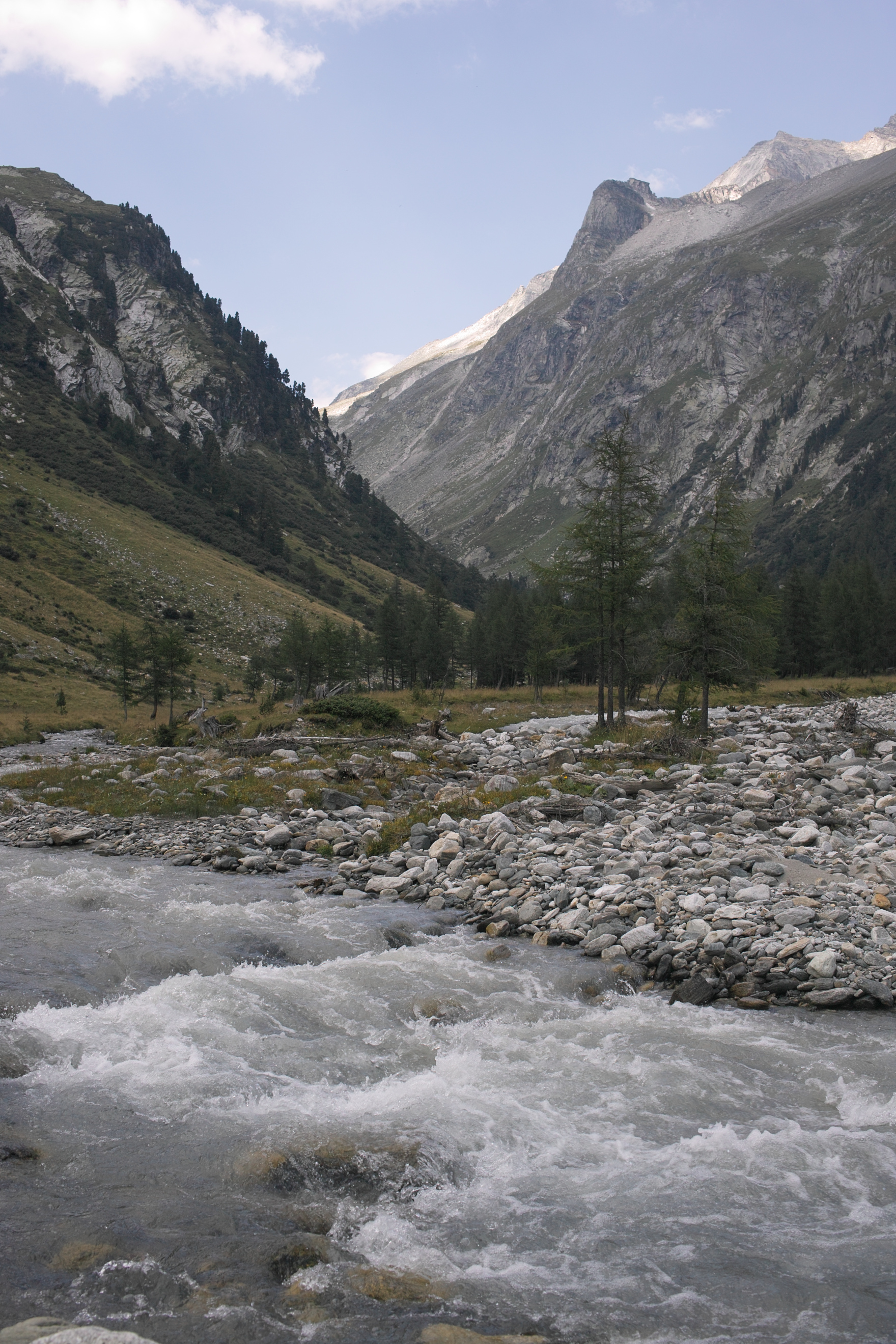
As you can see on the photo below, even in summer the peaks are covered with snow.
Timeseries data as input to the model are plotted in observed_timeseries.pdf. Temperature and precipitation are taken from CFSR, streamflow from GRDC.
Dorfertal catchment with main stream, photo taken in summer.
Except interception of precipitation (i.e., rainfall plus snowfall) by the vegetation, the model represents all main components of a hydrological system, where each component is modelled using simple equations. The figure below shows the model structure. The model has two storages, the snow storage and the subsurface storage. The latter represents all the water that is stored below the surface. The input of water is precipitation, the outputs from the system are streamflow and loss of water to the atmosphere. A number of fluxes is defined each defined by a particular equation. These equations use so called parameters, which are mostly assumed to be fixed. They are shown in red in the schematic. It is often hard to directly measure parameters and this is why they are ‘calibrated’. We will come back to this later.
An essential component in the model is the air temperature. As it is not measured for all pixels in the area, we use a time series of temperature observed at a certain reference elevation. As temperature mostly decreases with elevation, temperature is then estimated for each pixel using the digital elevation model (surface level of each pixel). For detailed model equations refer to the text below. Most important in this exercise is the snowmelt rate parameter which is the one that will be calibrated.
Schematic of the model. Reference elevation of temperature is in principle given by the dataset, but has some uncertainty and could be adjusted in calibration, which is why it is shown as a parameter here.
The equations below are evaluated for each grid cell, for all timesteps (time step is 1 day):
The air temperature (, degrees Celcius) above the surface is:
With, , the observed temperature (degrees Celcius); , the temperature lapse rate (degrees / m elevation); , the elevation of the land surface; , the reference elevation of the observed temperature.
Snowfall (, m equivalent water depth/day) is
With, , the observed precipitation (m/day).
Rainfall (, m/day) is
The rate of change in the snow depth (, m equivalent water depth) is
With, , meltrate parameter (degree day factor, m/(day degree)); , sublimation (m/day). The sublimation is equal to the loss of water to the atmosphere parameter (, m/day); if the snow depth becomes zero, sublimation becomes zero and loss of water to the atmosphere is taken from the subsurface water storage (see below).
The water flux available for infiltration () equals the sum of snowmelt and rainfall:
With, , the snow melt rate parameter (m/(day degree)). The actual infiltration (, m/day) is:
With, the infiltration capacity parameter (m/day).
Water in the subsurface is represented by (m), this is the amount of water stored below the surface, loosely defined as groundwater. Upward seepage from the subsurface (, m/day, loss of groundwater to the surface water) is:
With, , seepage parameter (/day). The rate of change in the groundwater is:
With, the loss to the atmosphere which is zero in case of snow cover (in which case loss to the atmosphere is taken from the snow cover).
The amount of surface runoff (m/day) generated is:
The streamflow is calculated for each day as the sum of in all the upstream pixels of a cell.
Inspect the script runoff.py. It is a standard PCRaster Python script except for the added capability to pass a parameter value to the actual model; the def__init__ statement takes an argument meltRateParameter which is passed when calling the model at the bottom of the script. At the bottom of the script is also some code that will be used for the calibration, which will be explained later on. The model simulates the same time span as given by observed_timeseries.pdf, i.e. three years.
Execute the model. Inspect the timeseries of maps created by the model; snow depth, snow (snow0000.001, snow0000.002, etc maps); subsurface storage, sub; and streamflow discharge, dis. For instance:
Do not forget to right-mouse click on the legend to plot the timeseries - if you click on the map you can then plot the timeseries for any location.
Question: Does the snowdepth at timestep 1 have a realistic value?
Yes, it is midsummer and snowdepth is thus close to zero.
Yes, it is midwinter but there was hardly any snowfall resulting in zero snowdepths.
No, it is assumed snowdepth is zero at the start as there is no information on the starting value.
No, it is assumed snowdepth is at a maximum at the start as there is no information on the starting value.
Correct answers: c.
Feedback:
The depth of the snow is unknown at the start, which is 1 january, i.e. midwinter. Of course there will be a considerable snowpack then. So simulation results for the first year at least should be considered a rough estimation. In the calibration later on we will use the first year to ‘spin up’ the model and from year two on data are used for the calibration.
Question: What is the mechanism determining larger amounts of streamflow in spring?
Snowmelt. The snowdepth is decreasing in spring causing high streamflow. In addition, peaks in streamflow occur due to direct rain.
Rainfall. The rainfall is seasonal with highest rain in winter and spring. In winter it falls as snow but in spring it falls as rain causing high streamflow.
Loss of water to the atmosphere. This changes over time, with highest losses in summer and winter, causing higher streamflow in spring (and autumn).
Wrong! Streamflow is highest in summer when precipitation falls as rain, which drains to the stream.
Correct answers: a.
Feedback:
Like most Alpine catchments the streamflow is mainly determined by the occurence of snowmelt. In spring, snowmelt is highest due to increasing temperatures. In summer and autumn most of the snow has disappeared and only rainfall contributes to streamflow (and flow from the groundwater). In winter there is hardly discharge as precipitation falls as snow, but there will be some baseflow from the groundwater.
Let’s now compared modelled streamflow with observed (measured) streamflow. Here we do so by importing the observed streamflow (at the measurement location) to the model and reporting it as a map. This is somewhat cumbersome but has the advantage that we can evaluate results with aguila.
Add the following to the bottom of the dynamic section:
Calculate the difference between modelled and observed streamflow (use the - operator, modelled minus observed).
Write this difference map to disk (report), use dMmO as output file name.
Write the observed discharge to disk (dis_obs), use dO as output file name.
Run the model and display dO, dMmO, and dis. Right-click on the legend to plot the timeseries and then click on the measurement location to retrieve the values at the this location in the timeseries.
Question: What is the main difference between modelled and observed streamflow?
The streamflow is overestimated in midwinter.
The streamflow is often too high in autumn.
The streamflow is often too low in spring and too high in summer.
The streamflow is often too high in spring and too low in summer.
Correct answers: c.
Feedback:
The streamflow is too high in summer and too low in spring. In other words, the high streamflows due to melting of the snow come too late in the season. The bottom part of the dynamic section should look like this:
# read observed dischargedis_obs=timeinputscalar('streamflow.txt',ifthen(self.sampleLocation,boolean(1)))# modelled minus observed dischargedisMmO=dischargeMetrePerSecond-dis_obs# write to diskself.report(disMmO,'dMmO')self.report(dis_obs,'dO')
 which is the one that will be calibrated.
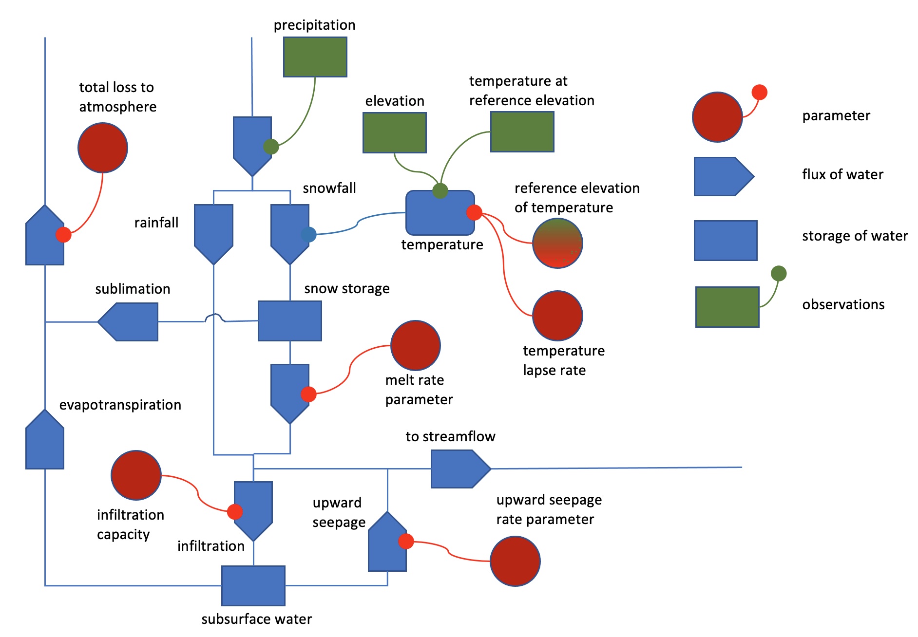
 , degrees Celcius) above the surface is:
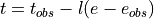
 , the observed temperature (degrees Celcius);
  , the temperature lapse rate (degrees / m elevation);
  , the elevation of the land surface;
  , the reference elevation of the observed temperature.
 , m equivalent water depth/day) is
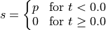
 , the observed precipitation (m/day).
 , m/day) is
 , m equivalent water depth) is
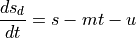
 , sublimation (m/day). The sublimation is equal to the loss of water to the atmosphere parameter (
 , m/day); if the snow depth
  ) equals the sum of snowmelt and rainfall:
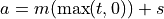
 , m/day) is:
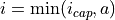
 the infiltration capacity parameter (m/day).
 (m), this is the amount of water stored below the surface, loosely defined as groundwater. Upward seepage from the subsurface (
 , m/day, loss of groundwater to the surface water) is:
 , seepage parameter (/day). The rate of change in the groundwater is:
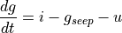
 in all the upstream pixels of a cell.