6.3. Calibration of a single parameter¶

6.3.1. Calibration using brute force¶

We will now calibrate the melt rate parameter with the brute force technique. Brute force means that we run the model multiple times, in a loop, each time with a parameter value taken from a predefined list of parameter values. The parameter values that gives the best fit with observed discharge is the ‘optimum’ value, i.e. the calibrated value.

But what is ‘best fit’? This can be defined with a goal function or objective function. Here we use the ‘mean squared error’:

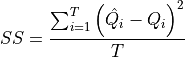
$SS = \frac{\sum_{i=1}^{T}\left ( \hat{Q_{i}}-Q_{i} \right )^2}{T}$

With, $SS$ , the value of the goal function; $\hat{Q_{i}}$ , modelled streamflow at timestep $i$ ; $Q_{i}$ , measured streamflow at timestep $i$ ; $T$ , the number of timesteps.

Open runoff_calibration_one_par.py. Again it is the same script as runoff.py but the reports to disk have been removed. Have a look at the lower part now. There, the observed streamflow is first read from disk and stored as an array named streamFlowObserved. This represents the $Q_{i}$ values in the equation above. The lowest part then calls the model (and passing the melt rate parameter value) which returns the modelled streamflow streamFlowModelled. At the bottom then the goal function above is evaluated for all timesteps. Note that it neglects the first year, which is the spin up time period required as snow cover is not yet realistic in this year.

If you run the model once, it prints the parameter value used and the objective function value.

Now modify the script such that it runs the model for a series of snow melt rate values, for instance from 0.0 up to 0.02, with a step size of 0.001. Note that you can first run it with a larger step and later on ‘zoom in’ to the correct value by narrowing the search range and using smaller steps. You will need to write a loop in Python, where you call the model each time with a different melt rate value. Store results in a text file and plot the response line, which is a plot of the parameter value (on the x-axis) vs. the goal function value (on the y-axis). The lowest point on this curve is the calibrated melt rate.

Question: What is the calibrated value of the melt rate parameter?

0.0089
0.0090
0.0060
0.0061

Correct answers: b.

Feedback:

The answer script is provided below. It writes a text file that you can plot with plotting program (e.g. spreadsheet) or with for instance matplotlib in Python. The matplotlib script is also provided below.

from pcraster import *
from pcraster.framework import *


# helper function 1 to read values from a map
def getCellValue(Map, Row, Column):
    Value, Valid=cellvalue(Map, Row, Column)
    if Valid:
      return Value
    else:
      raise RuntimeError('missing value in input of getCellValue')

# helper function 2 to read values from a map
def getCellValueAtBooleanLocation(location,map):
    # map can be any type, return value always float
    valueMap=mapmaximum(ifthen(location,scalar(map)))
    value=getCellValue(valueMap,1,1)
    return value


class MyFirstModel(DynamicModel):
    def __init__(self, meltRateParameter):
        DynamicModel.__init__(self)
        setclone('clone.map')

        # assign 'external' input to the model variable
        self.meltRateParameter = meltRateParameter 

    def initial(self):
        self.clone = self.readmap('clone')

        dem = self.readmap('dem')

        # elevation (m) of the observed meteorology, this is taken from the
        # reanalysis input data set
        elevationMeteoStation = 1180.0
        elevationAboveMeteoStation = dem - elevationMeteoStation
        temperatureLapseRate = 0.005
        self.temperatureCorrection = elevationAboveMeteoStation * temperatureLapseRate

        # potential loss of water to the atmosphere (m/day)
        self.atmosphericLoss = 0.002 

        # infiltration capacity, m/day
        self.infiltrationCapacity = scalar(0.0018 * 24.0)

        # proportion of subsurface water that seeps out to surface water per day
        self.seepageProportion =  0.06 

        # amount of water in the subsurface water (m), initial value
        self.subsurfaceWater = 0.0

        # amount of upward seepage from the subsurface water (m/day), initial value
        self.upwardSeepage = 0.0
 
        # snow thickness (m), initial value
        self.snow = 0.0

        # flow network
        self.ldd = self.readmap('ldd')

        # location where streamflow is measured (and reported by this model)
        self.sampleLocation = self.readmap("sample_location")

        # initialize streamflow timeseries for directly writing to disk
        self.runoffTss = TimeoutputTimeseries("streamflow_modelled", self, self.sampleLocation, noHeader=True)
        # initialize streamflow timeseries as numpy array for directly writing to disk
        self.simulation = numpy.zeros(self.nrTimeSteps())


    def dynamic(self):
        precipitation = timeinputscalar('precipitation.txt',self.clone)/1000.0
        temperatureObserved = timeinputscalar('temperature.txt',self.clone)
        temperature = temperatureObserved - self.temperatureCorrection

        freezing=temperature < 0.0
        snowFall=ifthenelse(freezing,precipitation,0.0)
        rainFall=ifthenelse(pcrnot(freezing),precipitation,0.0)

        self.snow = self.snow+snowFall

        potentialMelt = ifthenelse(pcrnot(freezing),temperature * self.meltRateParameter, 0)
        actualMelt = min(self.snow, potentialMelt)

        self.snow = self.snow - actualMelt

        # sublimate first from atmospheric loss
        self.sublimation = min(self.snow,self.atmosphericLoss)
        self.snow = self.snow - self.sublimation
   
        # potential evapotranspiration from subsurface water (m/day)
        self.potential_evapotranspiration = max(self.atmosphericLoss - self.sublimation,0.0)

        # actual evapotranspiration from subsurface water (m/day)
        self.evapotranspiration = min(self.subsurfaceWater, self.potential_evapotranspiration)

        # subtract actual evapotranspiration from subsurface water
        self.subsurfaceWater = max(self.subsurfaceWater - self.evapotranspiration, 0)

        # available water on surface (m/day) and infiltration
        availableWater = actualMelt + rainFall
        infiltration = min(self.infiltrationCapacity,availableWater)
        self.runoffGenerated = availableWater - infiltration

        # streamflow in m water depth per day
        discharge = accuflux(self.ldd,self.runoffGenerated + self.upwardSeepage)

        # upward seepage (m/day) from subsurface water
        self.upwardSeepage = self.seepageProportion * self.subsurfaceWater 

        # update subsurface water
        self.subsurfaceWater = max(self.subsurfaceWater + infiltration - self.upwardSeepage, 0)

        # convert streamflow from m/day to m3 per second
        dischargeMetrePerSecond = (discharge * cellarea()) / (24 * 60 * 60)
        # sample the discharge to be stored as timeseries file
        self.runoffTss.sample(dischargeMetrePerSecond)

        # read streamflow at the observation location 
        runoffAtOutflowPoint=getCellValueAtBooleanLocation(self.sampleLocation,dischargeMetrePerSecond)
        # insert it in place in the output numpy array
        self.simulation[self.currentTimeStep() - 1] = runoffAtOutflowPoint

nrOfTimeSteps=1461

# read the observed streamflow from disk and store in numpy array
streamFlowObservedFile = open("streamflow.txt", "r")
streamFlowObserved = numpy.zeros(nrOfTimeSteps)
streamFlowObservedFileContent = streamFlowObservedFile.readlines()
for i in range(0,nrOfTimeSteps):
    splitted = str.split(streamFlowObservedFileContent[i])
    dischargeModelled = splitted[1]
    streamFlowObserved[i]=float(dischargeModelled)
streamFlowObservedFile.close()


# function to create series of parameter values for which model is run
def createParValues(lower,upper,nrSteps):
    step = (upper - lower)/(nrSteps-1)
    return(numpy.arange(lower,upper + step, step))

# create melt rate parameters for which model is run
meltRateParameters = createParValues(0.0, 0.02, 21)
print('model will be run for values of melt rate: ', meltRateParameters)

f = open("calibration_one_par_results.txt", "w")

# calibrate melt rate 
for meltRateParameter in meltRateParameters:
    myModel = MyFirstModel(meltRateParameter)
    dynamicModel = DynamicFramework(myModel,nrOfTimeSteps)
    dynamicModel.setQuiet()
    dynamicModel.run()

    # obtain modelled streamflow
    streamFlowModelled = myModel.simulation
    # calculate objective function, i.e. mean of sum of squares and ignore first year
    SS = numpy.mean((streamFlowModelled[365:] - streamFlowObserved[365:])**2.0)
    print('meltrate: ', meltRateParameter, ', mean squared error: ', SS)
    f.write(str(meltRateParameter) + " " + str(SS) + "\n")

f.close()

import matplotlib.pyplot as plt

# read the calibration results file
file = open("calibration_one_par_results.txt", "r")
lines = file.readlines()

parValues = []
goalValues = []
for line in lines:
    splitted = str.split(line)
    parValues.append(float(splitted[0]))
    goalValues.append(float(splitted[1]))
file.close()

f = plt.figure()
plt.plot(parValues,goalValues)
plt.xlabel("parameter value")
plt.ylabel("goal function value")
f.savefig("plot_calibration_one_par_results.pdf")

6.3.2. Effect of observations used in calibration¶

In the previous example you used the last three years for calibration. Let’s see whether using a subset of the data for calibration has an effect of the calibrated value.

Rerun the calibration but now calibrate on the discharge of the last year alone (instead of using the last 3 years).

Question: What is the calibrated value of the melt rate parameter, when calibrating against discharge for the last year only?

0.011
0.012
0.014
0.018

Correct answers: c.

Feedback:

The melt rate calibrated for the last year is somewhat higher. There are many possible explanation for this: measurements errors, process-descriptions in the model that in some years are more representative for processes ocurring in the system modelled compared to other years, gradual changes over years in drivers of the system, and maybe more. In general it is always better to use a longer time span for calibration as this results in a calibration that is representative of the average system behaviour.

    # calculate objective function, i.e. mean of sum of squares and ignore first year
    SS = numpy.mean((streamFlowModelled[1095:] - streamFlowObserved[1095:])**2.0)
    print('meltrate: ', meltRateParameter, ', mean squared error: ', SS)