1.5. Neighbourhood operations: DEM and catchment analysis
1.5.1. Introduction
A neighbourhood operation relates the cell to its neighbours. The value of each cell is changed on basis of some kind of relation with neighbouring cells or flow of material (for instance water) from neighbouring cells. This chapter will cover neighbourhood operators for catchment analysis.
1.5.2. Creating slope and aspect maps
The slope operator generates a slope map on basis of a digital elevation model (a fraction: increase in height per distance in horizontal direction, in a 3 x 3 cells window). Try:
slopeMap = slope(topoMap) <Enter>
Display slopeMap and topoMap.
With the atan operator, the slope given as an angle is calculated. Type:
slopedegMap = atan(slopeMap) <Enter>
Apply the operator slope to slopeMap. Type:
slope2Map = slope(slopeMap) <Enter>
The slope2Map gives the change in slope (second derivative).
The aspect operator results in a map of slope aspect in 360 degrees (clockwise, North is to the top of the map and is 0 degrees). Type:
aspectMap = aspect(topoMap) <Enter>
1.5.3. Creating the local drain direction map
In different kinds of environmental studies, such as erosion, surface runoff and hydrological research, it is important to be able to delineate a river course and drainage area. Digital Elevation Models (such as topoMap) offer the possibility for automated extraction of catchment characteristics by creating a local drain direction map which gives the flow pattern over a DEM.
The lddcreate operator is used to generate a local drain direction map. Its syntax is: Result = lddcreate(dem, outflowdepth, corevolume, corearea, precipitation) where dem is the digital elevation model. The other input maps (or constant values) are so-called pit removing thresholds, these are explained later.
First, set the pit removing thresholds to zero:
ldd0Map = lddcreate(topoMap,0,0,0,0) <Enter>
Display topoMap and ldd0Map.
The lddcreate operator has determined for each cell the direction of the steepest (downhill) slope, which is the direction of local drainage. For each cell, the drain direction is assigned to the local drain direction map ldd0Map.
The cells with a black square at the edge of the map represent outflow points from the map (you may need to zoom in a bit to see them). There are two similar cells ldd0Map that are not at the edge. These are called pits. A pit cell is surrounded by cells at a greater elevation than the pit cell itself. As result, a pit cell cannot drain to a neighbouring cell. In PCRaster, the cells can be assigned unique nominal values with the pit operator. Try:
pit0Map = pit(ldd0Map) <Enter>
Display the maps, including topoMap (in one aguila command). Enlarge the window of pit0Map and check the elevations at and around pit cells by clicking with the mouse on these cells and reading the topoMap values from the data window.
You can find the downstream paths over a local drain direction map with the path operator. It uses an boolean input map. All cells that are downstream of a TRUE cell on the boolean map are assigned a boolean TRUE on the resulting map.
The map pointsMap contains some arbitrary points with a boolean value TRUE. Display pointsMap. After that, try:
pathzeroMap = path(ldd0Map,pointsMap) <Enter>
aguila(ldd0Map, pointsMap, pit0Map, pathzeroMap) <Enter>
Compare ldd0Map and path0Map. You will see that the paths stop at the pit cells on the local drain direction map.
Two kinds of pits may occur in a DEM. The first kind is caused by natural depressions and sinkholes in a landscape, see the Figure below.
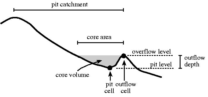
Figure: A sprinkling of the definitions used in theory of pit removing.
The pit will be at the cell with the smallest elevation in such a depression. The core of the pit is the area that will contain water if it would be filled with water until the overflow level is reached. The second kind of pits is introduced by the DEM itself. Due to the discretization of the elevation surface, the DEM is not an exact description of the landscape. As a result pits may occur on the DEM at locations without any real depressions in the landscape. These will have small and shallow cores on the DEM.
You can fill up the cores of all pits in a digital elevation model with the lddcreatedem operator. It generates a modified digital elevation model: the cores are filled up until the overflow level of the cores is reached. This can be compared with fluviatile sedimentation in the core depression until a maximum sedimentation level is reached (which is the overflow level of the pit). Type:
topomodiMap = lddcreatedem(topoMap,1e31,1e31,1e31,1e31) <Enter>
The 1e31 values effect that all cores will be filled up. To find the difference between topoMap and topomodiMap (which is the depth of the pit cores), type:
coredeptMap = topomodiMap - topoMap <Enter>
Question: What is the maximum depth of the largest core in the map (in metres)?
- 1.2
- 4.0
- 0.1
- 3.0
For further analysis it is necessary to remove the pits from the local drain direction map. This can be done by changing the pit remover thresholds given in the lddcreate operator. These are: the depth of the pit, outflowdepth; the volume or area of the pit core, corevolume and corearea respectively and the amount of rain needed to fill up the pit core, precipitation. With these thresholds you can define which pits must be removed from the map. Pits that have dimensions smaller than the threshold dimensions will be removed, pits that are larger than one (or more) of the thresholds remain in the local drain direction map. In this exercise, the pit depth (outflowdepth) will be used. Try:
ldd2Map = lddcreate(topoMap,2,1e31,1e31,1e31) <Enter>
This operation removes all pits except these with a depth that is larger than or equal to 2 metre. To find the pits in ldd2Map, type:
pit2Map = pit(ldd2Map) <Enter>
To remove all the pits, also the ones on the sides of the map, using very high threshold values (here 1e31, i.e. 10 to the power of 31), type:
lddMap = lddcreate(topoMap,10,1e31,1e31,1e31) <Enter>
Calculate the downstream paths and display:
pathMap = path(lddMap, pointsMap) <Enter>
You will see that all paths end at an outflow cell. For further analysis, lddMap will be used.
1.5.4. Catchment analysis and routing with the ldd map.
The catchments of all outflow points are determined with the catchment operator.
Use the pit operator to create a nominal map with the outflow points (call it outpoMap) from the study area, uniquely numbered. Use lddMap which you created in the previous exercise. Now, use catchment, type:
catchmsMap = catchment(lddMap,outpoMap) <Enter>
For each non zero cell value on outpoMap its catchment has been determined and all cells in its catchment have been assigned this non zero value on catchmsMap.
The main use of the local drain direction map is for routing of surface water in downstream direction. The accuflux operator transports an input of material (for instance rain) downstream over the local drain direction network to the outflow cells. It calculates for each cell the material flux over the ldd during transport. All material is transported. The syntax of accuflux is: Result = accuflux(ldd,material) where ldd is the local drain direction map and material is a map of scalar data type that contains the input of material.
The map rainstorMap gives the amount and distribution of rain (m3 per cell) that falls during a short rainstorm. Display the map. The discharge in the study area as a result of the rainstorm is calculated with the accuflux operator. It is assumed that no baseflow, no interception and no infiltration occurs. Type:
dischMap = accuflux(lddMap,rainstorMap) <Enter>
Display dischMap, rainstorMap and lddMap.
Question: What is the maximum value of the total discharge (m3) as a result of the thunderstorm?
- 1179.69
- 12.69
- 117969
- 1.17969
By taking the base10 logarithm of dischMap you can get a better picture of the spatial pattern of the discharge. Type:
dischlogMap = log10(dischMap) <Enter>
Alternatively, you could change the view of dischMap in Aguila, right click on its legend, select ‘Edit draw properties’ and change colour assignment to True logarithmic. You may need to set the minimum cutoff to 0.1 as log(0) is not possible.
The local drain direction map can also be used for the calculation of the upstream area map. The upstream area map contains for each cell the area of the cell its catchment (including the cell itself) that drains to the cell. The map is calculated with the accuflux operator. Instead of defining a material input for the material map in the operation, a map that contains for each cell the area of a cell (2500 m2) is used for material. As a result, this area ‘drains downstream’ and the catchment area of each cell is calculated. Try:
upareMap = accuflux(lddMap,2500)
Display upareMap and lddMap.