2.7. Direct neighbourhood operations
2.7.1. Discrete attributes: cellular automata
2.7.1.1. Initializing Game of Life
Game of Life is the best known cellular automata model. It models a population using Boolean valued grid cells, where True represents an alive cell and False a dead cell. Although it uses very simple deterministic transition rules it results in pretty unexpected results, as you will see.
The following transition rules are applied for each time step (generation). For each cell, the number of eight direct neighbourcells that is True (i.e., alive) is counted. This count is used to determine what happens with the cell in the time step:
- Birth: if the current cell is False and the count is 3, the current cell becomes True.
- Surivival: if (a) the count is 2, or (b) the count is 3 and the current cell is True, the current cell is left unchanged.
- Death: if the count is less than 2 or greater than 3, the current cell becomes False.
Go to the folder neighbourhood/life and open life.py. It is an almost empty model that runs only one time step. In a later phase you can increase the number of time steps. First you need to create an initial map of the distribution of alive cells. We assume that initially 10% percent of the cells is alive, at randomly chosen locations. In the initial section, add:
aUniformMap = uniform(1)
Store the result to disk and run.
Question: What is done by the uniform function?
- It draws a realization between 0 and 1, for each cell independently.
- It draws a realization between 0 and 1, for all cells at the same time.
- It sorts values on a map, and numbers the cells according to the order.
Now, use aUniformMap in a calculation to create the initial distribution of alive cells. You need the PCRaster function less than (<). Name the result of this calculation self.alive and write it to disk. Run and look at the results.
Question: What other (in addition to <) PCRaster operations did you use to create self.alive ?
ifthenifthenelseboolean- No other operation was required.
2.7.1.2. Implementing the update rules
To represent the Birth, Survival, and Death update rules, we need to add statements to the dynamic. To count the number of neighbouring cells that is True, the boolean map self.alive needs to be converted to a map with a scalar data type. In the dynamic, type:
aliveScalar = scalar(self.alive)
The function scalar assigns a scalar 1.0 to cells that are True on its input and 0.0 otherwise.
Now, add a statement to the dynamic calculating for each cell the number of neighbouring cells that is True. It should only count in a neighbourhood consisting of 8 direct neighbours (excluding the cell itself). You need to use at least the windowtotal function. Assign the result to the variable numberOfAliveNeighbours and write the result to disk. Run and compare the result with the map containing the alive cells (self.alive).
As a next step, let’s add the birth update rule. First create a Boolean map that is True for cells with 3 alive neighbours. Write to disk and check the results. Add another statement resulting in a map (birth) that returns True for cells with birth. You will need the functions pcrand and pcrnot.
Question: What statement did you use ?
birth=pcrnot(threeAliveNeighbours,pcrand(self.alive))birth=pcrand(self.alive,pcrnot(self.alive))birth=pcrand(self.alive,pcrnot(threeAliveNeighbours))birth=pcrand(threeAliveNeighbours,pcrnot(self.alive))
Now, add Survival. Add a statement that calculates a map (survivalA) that is True according to Survival rule (a) (i.e., count is 2). Also, calculate survivalB containing True according to Survival rule (b). Combine survivalA and survivalB to create a map (survival) with cells that survive.
Death does not need to be represented by a separate calculation, because it is implicit when Birth and Survival is combined.
As a last step, combine the maps birth and survival that updates the self.alive map. Write the self.alive map to disk at the bottom of the dynamic, and run the model again. By comparing the self.alive map in the initial and after the first timestep, check whether your script really follows the three update rules of Game of Life.
Now, run the model for 100 timesteps by changing the number of timesteps at the bottom of the script. Animate the self.alive maps.
Do you see similar patterns given at at http://mathworld.wolfram.com/GameofLife.html ?
Question: How did you combine the survivalA AND survivalB maps?
survival=pcrand(survivalA, survivalB)survival=pcror(survivalA, survivalB)survival=pcrxor(survivalA, survivalB)survival=survivalA + survivalB
2.7.2. Continuous attributes: spatial diffusion in vegetation modelling
2.7.2.1. A logistic growth model
Logistic growth of vegetation can be modelled as:
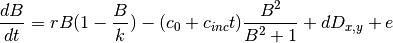
With:
 , biomass
 , growth rate (0.08)
 , carrying capacity (10)
 , initial grazing pressure (0.1)
 , increase in grazing pressure (0.00006)
 , dipsersion rate (0.01)
 , dispersion
 , random noise
In your exercises directory, go to the directory neighbourhood/growth and open growth.py. Program the logistic growth model assuming , , and are zero. The initial value of is 8.5. Use an explicit solution, which means that for each timestep, you calculate  according to the equation above and simply add it to . Use
 self.x as variable name for the biomass. Initialize it in the initial by typing:
self.x = spatial(scalar(8.5))
This is needed to tell PCRaster that self.x is a map (spatial) of data type scalar. Another hint: you can update the grazing pressure, i.e. the term  by typing in the dynamic:
self.c = self.c + self.cI
where c is the grazing pressure and cI is the increase in grazing pressure. In the initial you need to assign the initial value to grazing pressure.
Run the model for 2500 time steps and look at the result.
Question: What is the change in the biomass over time?
- It remains almost constant.
- It gradually increases.
- It increases exponentially.
- It gradually decreases and then drops quickly.
The observed change is known as a critical shift or critical transition in the literature. This means that the state of the ecosystem abruptly changes while the change in the driver is gradual. It is notably hard to predict such critical shifts, because the change in biomass is very small until the shift (here: abrupt decrease) occurs. Early warning signals have been described that change well ahead of the shift. One early warning signal is the spatial variance of the biomass. This can only be observed when some random noise is added to the biomass.
Add a statement to the dynamic that adds randomnoise to the biomass. You can create a map with random noise by typing:
randomNoise = normal(1)/10.0
Run the model again, and animate the map with the random noise, and the biomass.
Question: What is the effect of the random noise on the time series of maps of biomass?
- The time step for the critical shift differs spatially.
- The program hangs after some time steps due to random inputs.
- The resulting timing of the shift changes but is the same for all cells.
- The time series gets shorter.
Extend your script with statements that calculate the variance of the biomass map values. Remember that variance is:
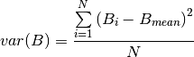
With:
 , a biomass value at a grid cell,
 , the mean biomass value of all grid cells,
 , the number of grid cells.
First, calculate , using maptotal, and note that the map is 40 by 40 cells. Use this map containing the mean value to calculate a map with the variance of biomass. The calculation needs to be done each time step, so add the statements to the dynamic. Store the output, run the model, display, and display the time series of variance.
Question: What is the change in the variance over time? Do you think it can be use to detect the upcoming downward shift in biomass?
- It decreases immediately, so it cannot be used to forecast the shift, which occurs much later.
- It increases immediately, so it cannot be used to forecast the shift, which occurs much later.
- It decreases well ahead of the shift, so it can be used to forecast the shift.
- It increases well ahead of the shift, so it can be used to forecast the shift.
2.7.2.2. Diffusion of biomass
Thus far, we neglected spatial interactions in the model. To represent clonal growth and other dispersal mechanisms of biomass, the model presented in the previous section includes dispersion  . It is calculated as:

With,
, diffusion term at a cell located at (x,y), , biomass at a direct neighbour in the negative y direction,
 , the number of direct neighbouring cells.
For all cells except cells at the edge of the map,  is equal to four neighbours, however at the edge cells one neighbour is missing, so we need to adjust here. In PCRaster Python, you can represent the equation by typing in the dynamic:
diffusion = self.d*(window4total(self.x)-self.numberOfNeighbours*self.x)
The window4total function sums the cell values of the four direct (top, right, bottom, left) neighbouring cells, self.d is the diffusion or dispersion rate (0.01). In the initial you need to calculate:
self.numberOfNeighbours = window4total(spatial(scalar(1)))
You also need to assign 0.01 to self.d in the initial. Add these statements to the model, such that diffusion is added to the biomass for each time step. Run the model and animate the biomass maps, using timeseries plots to evaluate the results.
Question: As you can see, the diffusion process results in patches of lower and higher biomass. What happens with the patch size over time (e.g. compare the pattern at the start of the model run, with the pattern just before the shift towards a lower biomass)?
- The patch size increases over time.
- The patches change, but the size stays the same.
- The patch size decreases over time.